Abdominal imaging at 3T: Challenges and solutions

Dr. Chang is Assistant Professor, Department of Diagnostic Imaging, Warren Alpert Medical School of Brown University and Rhode Island Hospital, Providence, RI; and Dr. Kamel is Associate Professor and Section Chief of Body and Cardiovascular MRI, Department of Radiology and Radiological Sciences, The Johns Hopkins University School of Medicine. Baltimore, MD.

Since the first 3 Tesla (3T) magnetic resonance imaging (MRI) scanners were approved for clinical use by the U.S Food and Drug Administration (FDA) in 2002, the use of 3T imaging has shown a gradual increase, especially for neuroradiologic and musculoskeletal studies. The theoretical advantages and promises of higher field imaging have greatly benefited many neurologic and musculoskeletal applications and potentially can improve imaging in the abdomen and pelvis as well. However, growth in the use of 3T in body imaging has been hampered due to problems related to more prominent artifacts occurring within the larger field of view of abdominal andpelvic studies.

This article will discuss the theoretical advantages of imaging at higher field strength as compared with 1.5T systems and the current imaging standards for body MRI. This article also discusses challenges related to imaging at 3T and various strategies that may be employed to solve them.

Signal-to-noise

The central promise of imaging at higher field strengths lies in an increased number of protons aligned with the stronger static magnetic field,contributing to greater signal and a higher signal-to-noise ratio (SNR). When 3T is compared with 1.5T, the SNR should theoretically double. However, the actual realized gain is less than this due to several factors including physiological noise, FDA-imposed specific absorption rate (SAR) limits (discussed below), inadequate scanner hardware, software optimization for 3T, radiofrequency (RF) field inhomogeneity, and increased susceptibility effects. Nevertheless, the benefit of a higher SNR can be used to increase spatial and temporal resolution, orsome combination of both.

T1 relaxation

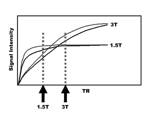
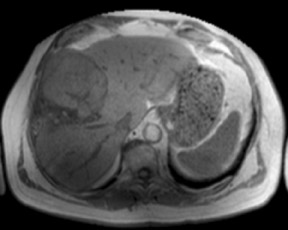
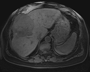
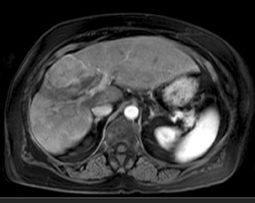
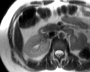
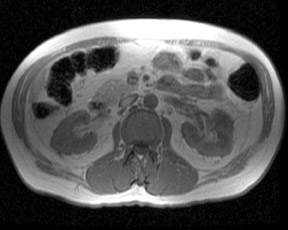
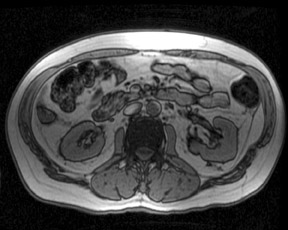
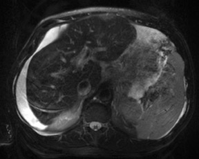
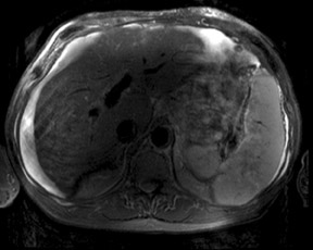
An increase in field strength leads to a prolongation of T1 relaxation time.¹ When comparing signal intensities of soft tissues at 3T and 1.5T, use of similar imaging parameters may lead to a significant decrease in relative soft-tissue contrast at 3T. A longer pulse repetition time (TR) may be required to generate a similar degree of soft tissue contrast (Figures 1 and 2).²

While decreased, unenhanced soft-tissue contrast may be compensated with a longer TR, this change leads to longer imaging time and is limited by the length of a single breath-hold. Another possible solution is the use of an inversion recovery preparatory pulse to accentuateT1 contrast. Magnetization preparation pulses,as have been used in MR angiography (MRA), can also aid in generating T1 contrast.^3,4 Short echo time (TE) gradient echo techniques have been successfully utilized as well. In addition, the use of parallel imaging can greatly shorten imaging time.

Gadolinium contrast effects

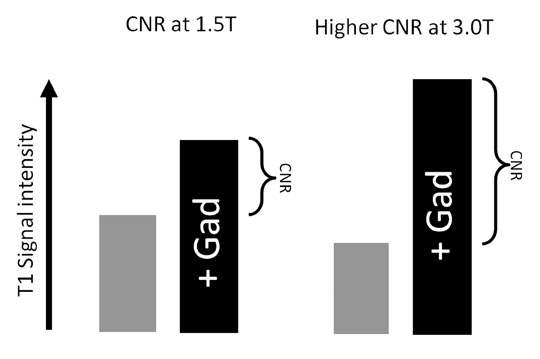
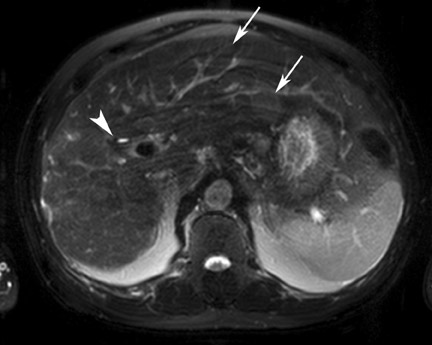
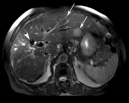
Although T1 relaxation times of soft tissues generally increase with a higher magnetic field strength, the relative T1 shortening effects of contrast agents, such as gadolinium, remain unchanged leading to more pronounced contrast enhancement of gadolinium-based contrast agents (GBCA) upon a background of tissues with longer T1 relaxation time. This wider dynamic range of effect leads to a higher contrast to noise ratio (CNR) with increasing field strength (Figures 3 and 4). A higher CNR results in improved lesion conspicuity at 3T, compared with lower field strengths, as well as improved contrast on MRA when using a similar dose of gadolinium.⁵ This effect raises the possibility for potentially halving the contrast dose at 3T compared with 1.5T, an issue of greater relevance in this age of increased awareness ofthe risks for nephrogenic systemic fibrosis.^6,7

T2 and T2* relaxation times

While changes in T1 relaxation time are well understood with an increase in field strength, the effects of 3T on T2 relaxation times are not as predictable. For most soft tissues, T2 relaxation times decrease slightly, whereas for fat, T2 relaxation times increase slightly.¹ Fluid T2 relaxation times do not significantly change when moving from 1.5T to 3T. However, the overall increase in SNR at 3T is more pronounced on T2-weighted (T2W) imaging compared with T1-weighted (T1W) imaging as a longer TR allows for more recovery of longitudinal magnetization. Sequences such as single-shot fast spin-echo (SSFSE) and half-Fourier acquisition single-shot turbospin-echo (HASTE) show significant increases in SNR and resulting improved lesion and fluid conspicuity at 3T (Figure 5). This increased SNR has also been used to boost spatial resolution, especially for techniques such as 3D MR cholangiopancreatography (MRCP).

While changes in T2 relaxation time are not as predictably affected with increases in field strength, T2* relaxation times are approximately halved with a doubling in field strength from 1.5T to 3T due to a doubling of magnetic susceptibility.^8,9 This effect significantly influences gradient-echo–based pulse sequences including echoplanar imaging. While problems related to field inhomogeneity may become more significant, these same effects serve to improve signal in techniques dependent on these susceptibility effects. Studies utilizing blood oxygen level dependent phenomenon (BOLD), such as functional MRI, show significant increases in signal sensitivity with higher field strength. While these studies are typically used in functional imaging of the brain, this technique has shown some early promise in abdominal imaging as well.¹⁰ Similarly, superparamagnetic iron oxide contrast (SPIO) may also make T2-hyperintense masses more conspicuous at 3T by more thoroughly suppressing signal in the background liver parenchyma.^11,12

As magnetic susceptibility effects are directly proportional to the field strength, higher field imaging is more sensitive to detection of gas, items such as surgical clips, and areas of iron deposition in solid organs. However, this effect also leads to areas of artifactual signal loss. Resultant areas of image distortion and loss of signal are most pronounced in and around areas containing gas or paramagnetic substances such as hemosiderin (Figure 6). These susceptibility artifacts may be mitigated through use of parallel imaging to shorten TE. This approach has already shown success in diffusion-weighted imaging (DWI) of the brain at 3T.^13,14

Chemical shift effects

Chemical shift effects are more pronounced with increases in field strength. Chemical shift effects of the first kind refer to differences in precession frequency between fat and water protons. The chemical shift between fat and water directly correlates to field strength and doubles to 440 Hz at 3T compared with 220 Hz at 1.5T. This alteration proportionally increases misregistration artifacts at interfaces between fat and water protons in the frequency encoding direction. The effect is doubled at 3T compared with 1.5T (Figure 7). However, the wider spectral separation between water and fat allows for more selective fat suppression limited only by magnetic field inhomogeneity at 3T. The improved spectral resolution available at 3T also allows for more robust MR spectroscopy with more discrete and quantifiable metabolite peaks.^15,16 The increased SNR available at 3T also permits faster and/or higher spatial resolution MR spectroscopy.

The more pronounced misregistration artifacts associated with chemical shift effects of the first kind can be counteracted through increased bandwidth. However, this is not without some penalty in diminished SNR. For example, moving from 1.5T to 3T imaging, a doubling of bandwidth is required to fully accommodate the doubled chemical shift artifact and results in a 29% decrease in SNR. The ability to increase bandwidth is also limited by gradient coil strength.

Chemical shift artifacts of the second kind are also known as “India ink” or phase cancellation artifacts and relate to the cancellation of signal in voxels containing both water and fat protons at TEs where fat and water protons are out-of-phase relative to each other. These TEs are shorter at higher field strengths and are halved at 3T when compared with 1.5T.¹⁷ At 3T, the in-phase and out-of-phase TEs are approximately 1.1 ms and 2.2 ms, respectively (Figure 8). Many 3T gradient coils are not capable of imaging with a TE as short as 1.1 ms, necessitating acquisition of the next-in-phase TE at around 3.3 ms, particularly if using a dual-echo approach to in-phase/out-of-phase imaging. However, imaging the in-phase echo at a TE longer than the earliest out-of-phase TE of 2.2 ms does not allow for differentiating signal drop out related to intravoxel fat from magnetic susceptibility effects. While 2 separate pulse sequences could be used rather than a dual-echo approach, this prolongs imaging time and may also raise potential problems related to lack of image co-registration. One potential advantage of a shorter out-of-phase TE at 3T is faster pulse sequences for MRA.

Diffusion weighted imaging

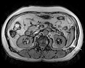
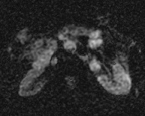
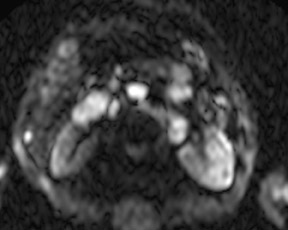
DWI also benefits from increased SNR at 3T. This translates to increased sensitivity to areas of restricted diffusion (Figure 9). DWI, however, is limited by the increased magnetic susceptibility artifacts present at 3T and the related areas of image distortion, particularly in areas of the abdomen and pelvis adjacent to air such as the lung bases and gas-filled loops of bowel. Susceptibility effects at 3T may be substantially decreased through the use of parallel imaging techniques such as SENSE, iPAT (Siemens Healthcare, Malvern, PA), GRAPPA (Siemens), and ASSET (GE Healthcare, Chalfont St. Giles, UK). These parallel imaging techniques limit susceptibility artifacts through shortening TE and overall imaging time. Such approaches have already been introduced in brain imaging for the detection of stroke.^13,14

Specific absorption rate

The specific absorption rate (SAR) for clinical imaging of the abdomen is limited by the FDA and the International ElectrotechnicalCommission (IEC) to either 4 W/kg over a 15 min period or 8 W/kg over a 5 min period in an effort to prevent soft tissue heating by >1 degree Celsius. This limitation holds regardless of magnetic field strength and becomes a very realistic limitation at 3T. The relationship of the SAR to various imaging parameters can be summarized in the mathematical relationship:

SAR ∝ B₀ ² α² DV

The SAR is proportional to the square of the magnetic field strength (B₀) and the square of the flip angle (α) and is directly proportional to the duty cycle (D) and the volume of the patient imaged (V).Duty cycle represents the maximum amount of time a gradient system may be run at maximum power and is directly related to the number and spacing of RF pulses.

As a doubling of field strength from 1.5T to 3T results in a quadrupling of the SAR, if no other parameters are changed, significant compromises in other energy deposition parameters are necessary at 3T in order to adhere to mandated SAR limits. These limits are particularly relevant to RF-intensive pulse sequences such as fast spin echo, steady-state free precession, and 3D gradient echo.

As SAR is proportional to the square of the flip angle, decreases in the flip angle utilized at 3T can significantly decrease energy deposition. However, the cost of decreasing flip angles on gradient echo sequences is a further loss in T1 contrast and a decrease in background signal suppression on MR angiography. More advanced techniques to reduce the flip angles used at 3T include RF refocusing pulse sequences such as flip-angle sweep, hyperechoes, and smooth transitions between pseudo steady states (TRAPS).^18,19 These techniques employ variable refocusing angles throughout the course of the pulse sequence to significantly reduce energy deposition at a cost of mildly decreased SNR.

Changes in the duty cycle can also be used to manage SAR issues at higher field strengths. Prolongation of the TR between pulse excitations has already been discussed and is one approach that can decrease RF energy deposition at a cost of increased imaging time. Another approach includes using longer and lower amplitude RF pulses, however, this necessitates a longer TE. The number of RF pulses can also be decreased by decreasing the number of phase-encoding and/or slice-select steps at a cost of lower spatial resolution, increased slice thickness, and/or a decreased field of view. An alternative strategy to more efficiently manage SAR includes alternating the use of high and low SAR sequences throughout the course of an MR examination. The use of parallel imaging at 3T can significantly decrease SAR by accelerating and shortening imaging time and reducing the number of RF excitations at a cost of some SNR.²⁰ The effect of a decrease in SNR on image quality is less pronounced at 3T than it is at 1.5T. Finally, improving RF field homogeneity (B₁) and RF efficiency through improved RF shimming and the use of multi-transmitter coils is a more recent approach that has been incorporated in many newer clinical 3T MR scanners. Further development of combined transmit-and-receive coils should also improve RF efficiency.²¹

Finally, decreasing the imaging volume can also decrease SAR. While this is usually a fixed variable for a particular scanner that depends on the width and diameter of the imaging bore, the recent development of shorter more “open” bore architectures may potentially decrease SAR at 3T. Disadvantages of these shorter bores include a more limited field of view in the craniocaudal plane, more pronounced image distortion at the field of view edges and a more inhomogeneous magnetic field.

Field inhomogeneity and dielectric effects

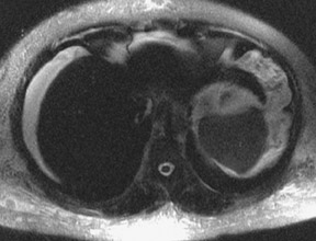
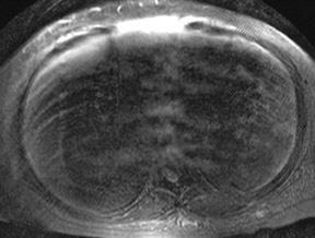
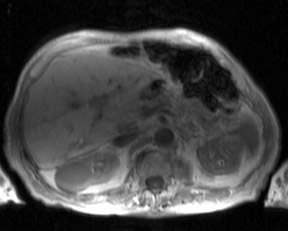
As was previously discussed, significantly increased sensitivity to T2* effects can lead to substantial susceptibility artifacts and wider variations in magnetic field homogeneity at 3T. Similarly, another major contributing factor in signal intensity variations across an image are standing wave or dielectric effects that are more pronounced at 3T than at lower field strengths. At lower field strengths, the RF wavelength corresponding to the Larmor frequency of water protons is significantly longer than the typical diameter of a patient’s torso. For example, at 1.5T, the Larmor frequency of water is 64 MHz corresponding to an RF wavelength of 52 cm. At 3T, however, the Larmor frequency of water protons doubles to 128 MHz necessitating a concomitant shortening of the RF pulse excitation wavelength to 26 cm, a measure closer to the typical dimensions of an abdomen or pelvis. This effect results in an increase in standing waves, defined as areas of constructive and destructive interference, that lead to large variations in local signal intensity across an image.²² This “dielectric shading” effect is more apparent with a larger body habitus or in a more ellipsoid body cross section.²³ Large volumes of intra-abdominal fluid such as ascites or amniotic fluid can also contribute shielding effects that can produce large signal voids in the central torso (Figure 10).²⁴ Fast spin echo sequences are typically affected more than gradient echo sequences. This artifact is a major reason why adoption of 3TMR imaging has been slower in body imaging compared with smaller field of view MR examinations such as the brain and joints.

Multiple approaches have been used to address issues related to field inhomogeneity and dielectric shading. The use of parallel imaging to shorten acquisition time can decrease susceptibility effects. Decreases in voxel size can also limit the amount of intravoxel dephasing. Shortening of TE can also decrease magnetic susceptibility effects, but may require an increase in bandwidth or a decrease in SNR.

To address dielectric effects, the use of dielectric pads or “RF cushions,” containing a conductive fluid or gel placed anterior to the torso, can partially alleviate standing wave artifacts. Many recent advances in scanner hardware with improvements in B₀ and RF shimming as well as RF transmission efficiency have led to more homogeneous B₀ and B₁ (RF) fields at 3T and significantly decreased dielectric shading, particularly in body imaging.

Safety

The safety of an implanted medical device at 1.5T does not imply safety at 3T. Fewer devices have been approved for MR imaging at 3T than at 1.5T; however, further testing is ongoing. The reason why device safety remains a great concern at 3T is due to the proportional increase in the translational attraction and torque on implanted devices that accompany an increase in magnetic field strength.²⁵ These forces are even more pronounced with short-bore magnets due to increased spatial gradients and resulting increases in deflection angles.²⁶ As clinical experience continues to build with 3T imaging more devices will eventually be approved. Similarly, due to lack of experience, the safety of 3T MRI remains unproven in the pregnant patient.

With an increase in field strength there is an increase in the size of the magnetic fringe field. At 3T this requires either a larger 5 Gauss safety margin or an increase in the use of active shielding.

Cost and design considerations

As with any new technology, the cost of 3T MRI scanners has been gradually decreasing over time. However, the initial cost of a 3T scanner has continued to be roughly twice the cost of a comparable 1.5T scanner. Not only is the initial outlay higher, but the continued cost of maintenance for a higher field superconducting magnet also tends to be higher due to faster cryogen consumption. Nevertheless, a few manufacturers have improved cryogen reliquification efficiency to the point of “zero boil off,” however, the larger cryogen reliquifiers required also increase costs associated with higher power consumption.

The larger fringe field of a higher field strength magnet necessitates a larger 5 Gauss safety margin that may require a larger room for a 3T system or involve the use of active shielding, which also adds to initial and ongoing operational expenses. Another site concern for a 3T magnet includes the approximately doubled weight, compared with comparable lower field systems. System noise generation is another factor to consider, although use of acoustic shielding has diminished this problem. Lastly, fewer RF coils are available for 3T than for 1.5T scanners, although more coils are being introduced each year. At this point in time, RF coils designed for 3T scanners also tend to be 50% to 100% more expensive than their 1.5T counterparts, although prices are expected to decrease over time.

Conclusion

3T imaging is becoming more commonplace as relative costs and the number of imaging applications increase. Adoption of 3T in body imaging has been slower than in neurologic and musculoskeletal imaging in great part related to the various challenges that imaging at a higher field strength introduces in abdominal and pelvic studies.

There are significant differences in the behavior of protons at 3T compared with lower field strengths. Both T1 and T2* relaxation times are significantly affected by a boost in magnetic field strength. Specific absorption rates have also become a much more significant concern at 3T as energy deposition quadruples when compared with 1.5T. Chemical shift artifacts, as well as magnetic and RF field in homogeneities, are also important considerations at 3T. Standing wave or dielectric shading artifacts are of particular concern for abdominal imaging at 3T due to the larger field of view compared with that for the brain and extremities. A wide variety of strategies can and have been successfully employed to address many of these issues, resulting in significant improvements in image quality since its clinical introduction earlier this decade.

In addition to the imaging related challenges, there are significant safety, cost and design considerations in the purchase and maintenance of a 3T MR scanner. The ultimate tradeoff for dealing with the many challenges of imaging the abdomen at 3T is a substantial boost in SNR, which can be used towards improving spatial, temporal and spectral resolution. This boost in SNR can also benefit many specific abdominal applications such as MR angiography, MR cholangiopancreatography, DWI, and MR spectroscopy.

Acknowledgements

Special thanks to David A. Bluemke, Ihab R. Kamel, and Katarzyna J. Macura for their help and guidance during preparation of a previous iteration of this topic originally published in Radiographics.²⁷

REFERENCES

1. de Bazelaire CM, Duhamel GD, Rofsky NM, Alsop DC. MR imaging relaxation times of abdominal and pelvic tissues measured in vivo at 3T: Preliminary results. Radiology.2004;230:652–659.
2. Bushberg J. In: The Essential Physics of Medical Imaging.2nd ed. Philadelphia, PA: Lippincott Williams & Wilkins, 2002:xvi,933.
3. Lee JH, Garwood M, Menon R, et al. High contrast and fast three-dimensional magnetic resonance imaging at high fields. Magn Reson Med. 1995;34:308–312.
4. Wolff SD, Eng J, Balaban RS. Magnetization transfer contrast: method for improving contrast in gradient-recalled-echo images. Radiology. 1991;179:133–137.
5. Elster AD. How much contrast is enough? Dependence of enhancement on field strength and MR pulse sequence. Eur Radiol.1997;7 Suppl 5:276–280.
6. Fukatsu H. 3T MR for clinical use: update. Magn Reson Med Sci. 2003;2:37-45.
7. Krautmacher C, Willinek WA, Tschampa HJ, et al. Brain tumors: full- and half-dose contrast-enhanced MR imaging at 3T compared with 1.5 T—Initial Experience. Radiology.2005;237:1014–1019.
8. Lewin JS, Duerk JL, Jain VR, et al. Needle localization in MR-guided biopsy and aspiration: Effects of field strength, sequence design, and magnetic field orientation. AJR Am J Roentgenol. 1996;166:1337–1345.
9. Olsrud J, Latt J, Brockstedt S, et al. Magnetic resonance imaging artifacts caused by aneurysm clips and shunt valves: dependence on field strength (1.5 and 3 T) and imaging parameters. J Magn Reson Imaging. 2005;22:433–437.
10. Li LP, VuAT, Li BS, et al. Evaluation of intrarenal oxygenation by BOLD MRI at 3T. J Magn Reson Imaging. 2004;20:901–904.
11. Chang JM, Lee JM, Lee MW, et al. Superparamagnetic iron oxide-enhanced liver magnetic resonance imaging: Comparison of 1.5 T and 3T imaging for detection of focalmalignant liver lesions. Invest Radiol. 2006;41:168–174.
12. Simon GH, Bauer J, Saborovski O, et al. T1 and T2 relaxivity of intracellular and extracellular USPIO at 1.5T and 3T clinical MR scanning. Eur Radiol. 2006;16:738–745.
13. Kuhl CK, Gieseke J, von Falkenhausen M, et al. Sensitivity encoding for diffusion-weighted MR imaging at 3T:Intraindividual comparative study. Radiology. 2005;234:517–526.
14. Kuhl CK, Textor J, Gieseke J, et al. Acute and subacute ischemic stroke at high-field-strength (3.0-T) diffusion-weighted MR imaging: Intraindividual comparative study.Radiology. 2005;234:509–516.
15. Gruetter R, Weisdorf SA, Rajanayagan V, et al. Resolution improvements in in vivo 1H NMR spectra with increased magnetic field strength. J Magn Reson. 1998;135:260–264.
16. Katz-Brull R, Rofsky NM, Lenkinski RE. Breathhold abdominal and thoracic proton MR spectroscopy at 3T. Magn Reson Med. 2003; 50:461–467.
17. Wehrli FW, Perkins TG, Shimakawa A, Roberts F. Chemical shift-induced amplitude modulations in images obtained with gradient refocusing. Magn Reson Imaging.1987;5:157–158.
18. Hennig J, Scheffler K. Hyperechoes. Magn Reson Med. 2001;46:6–12.
19. Hennig J, Weigel M, Scheffler K. Multiecho sequences with variable refocusing flip angles: Optimization of signal behavior using smooth transitions between pseudo steadystates (TRAPS). Magn Reson Med. 2003;49:527–535.
20. Pruessmann KP. Parallel imaging at high field strength: Synergies and joint potential. Top Magn Reson Imaging. 2004;15:237–244.
21. Vaughan JT, Adriany G, Snyder CJ, et al. Efficient high-frequency body coil for high-field MRI. Magn Reson Med. 2004;52:851–859.
22. Collins CM, Liu W, Schreiber W, et al. Central brightening due to constructive interference with, without, and despite dielectric re-sonance. J Magn Reson Imaging.2005;21:192–196.
23. Hussain S. Body MR Imaging: Current Practice and Future Horizons. In: Scientific Assembly and Annual Meeting of Radiological Society of North America. Chicago, IL,2006.
24. Merkle EM, Dale BM, Paulson EK. Abdominal MR imaging at 3T. Magn Reson Imaging Clin N Am. 2006;14:17–26.
25. Shellock FG. Biomedical implants and devices: Assessment of magnetic field interactions with a 3.0-Tesla MR system. J Magn Reson Imaging. 2002;16:721–732.
26. Shellock FG, Tkach JA, Ruggieri PM, Masaryk TJ. Cardiac pacemakers, ICDs, and loop recorder: Evaluation of translational attraction using conventional (“long-bore”) and “short-bore” 1.5- and 3.0-Tesla MR systems. J Cardiovasc Magn Reson. 2003;5:387–397.
27. Chang KJ, Kamel IR, Macura KJ, Bluemke DA. 3.0-T MR imaging of the abdomen: Comparison with 1.5 T. Radiographics. 2008;28:1983–1998.